Learning to create geometry unions

Motivation

I was asked at work if it were possible to aggregate polygons, that share boundries, in a bigger group. Since I am a novice when it comes to spatial analysis, I responded that “someone must have done it, I shall search and learn”. This lead me to the book Geocomputation with R. It has more than all I need. Highly recommended. What I liked about the book is that someone who has limited knowledge of spatial analysis but is comfortable with basic tidyverse operations can approach parts of this book as and when needed.

Actual geometries and how I want it to be

library(tidyverse)

## -- Attaching packages ----------

## v ggplot2 3.3.1     v purrr   0.3.4
## v tibble  3.0.1     v dplyr   1.0.0
## v tidyr   1.0.3     v stringr 1.4.0
## v readr   1.3.1     v forcats 0.5.0

## Warning: package 'ggplot2' was built under R version 3.6.3

## Warning: package 'tibble' was built under R version 3.6.3

## Warning: package 'purrr' was built under R version 3.6.3

## Warning: package 'dplyr' was built under R version 3.6.3

## Warning: package 'forcats' was built under R version 3.6.3

## -- Conflicts -------------------
## x dplyr::filter() masks stats::filter()
## x dplyr::lag()    masks stats::lag()

library(sf)

## Warning: package 'sf' was built under R version 3.6.3

## Linking to GEOS 3.8.0, GDAL 3.0.4, PROJ 6.3.1

library(here)

## here() starts at D:/R projects/Personal Website

library(patchwork)

spatial_data <- read_sf(here("content","post","BlocksClean.shp"))

As an example, I will be using the block (an admistrative unit) level shape file of the Siwan distirct in Bihar.

Here is how the data looks.

head(spatial_data)

## Simple feature collection with 6 features and 3 fields
## geometry type:  MULTIPOLYGON
## dimension:      XY
## bbox:           xmin: 84.1725 ymin: 26.1525 xmax: 84.77702 ymax: 26.37694
## geographic CRS: WGS 84
## # A tibble: 6 x 4
##   NAME      DISTRICT                                          geometry Anumandal
##   <chr>     <chr>                                   <MULTIPOLYGON [°]> <chr>    
## 1 Nautan    Siwan    (((84.17898 26.37034, 84.17906 26.37038, 84.1798~ Siwan Sa~
## 2 Siwan     Siwan    (((84.32079 26.33337, 84.32163 26.33337, 84.3244~ Siwan Sa~
## 3 Barharia  Siwan    (((84.35839 26.37073, 84.35863 26.37124, 84.3590~ Siwan Sa~
## 4 Goriakot~ Siwan    (((84.54271 26.30274, 84.5432 26.30263, 84.54771~ Maharajg~
## 5 Lakri Na~ Siwan    (((84.62733 26.30347, 84.62758 26.30344, 84.6298~ Maharajg~
## 6 Basantpur Siwan    (((84.59785 26.17777, 84.59704 26.17799, 84.5962~ Maharajg~

The NAMEcolumn has the name of the block. The DISTRICT, this wont be needed, column shows the district. The Anumandal column shows which anumandal (larger admistrative unit thatn a block) does a given block fall under.

This is how the shape file looks when plotted.

spatial_data %>% 
  ggplot()+
  geom_sf()+
  geom_sf_text(aes(label = str_sub(NAME,1,4)))+
  theme_minimal()

## Warning in st_point_on_surface.sfc(sf::st_zm(x)): st_point_on_surface may not
## give correct results for longitude/latitude data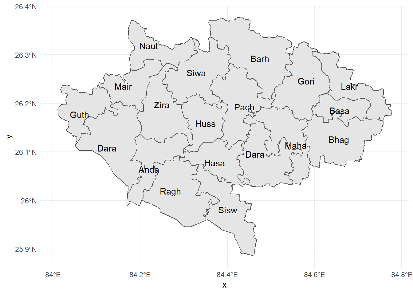

All the blocks are plotted, however, I want to agregate boundries of those blocks that fall under the same Anumandal.

Let fill in the shape with colours acording to the Anumandal to which the block belongs.

spatial_data %>% 
  ggplot()+
  geom_sf(aes(fill = Anumandal))+
  geom_sf_text(aes(label = str_sub(NAME,1,4)))+
  theme_minimal()

## Warning in st_point_on_surface.sfc(sf::st_zm(x)): st_point_on_surface may not
## give correct results for longitude/latitude data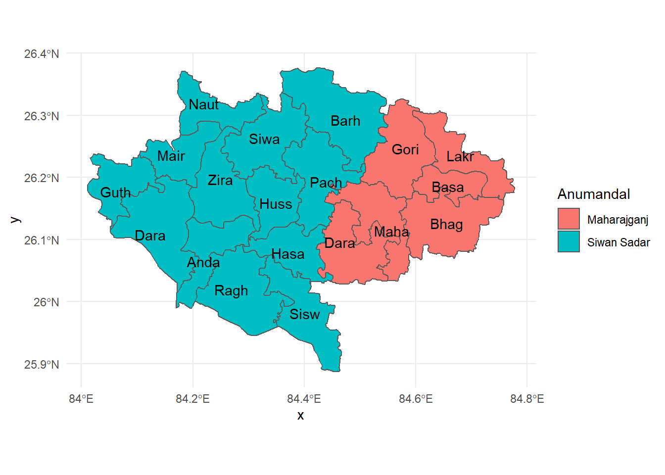

Above shown map is close to what I am aiming for.

Let us see how it can be done by following the instructions in the book Geocomputation with R.

Creating Geometric Unions

I am refereing to the sections 3.2.2 and 5.2.6 of the book. An interesting note on aggregate() function that I read is reporduced below.

“aggregate() is a generic function which means that it behaves differently depending on its inputs. sf provides the method aggregate.sf() which is activated automatically when x is an sf object and a by argument is provided”

Another important thing to note is also reporduced below.

“Behind the scenes, both aggregate() and summarize() combine the geometries and dissolve the boundaries between them using st_union()”

Here is a code chunk to attemmt and dissolve the relevant Block geometries into Anumandal geometries.

spatial_data %>% 
  group_by(Anumandal) %>% 
  summarise(
    Number_of_Blocks = n()
  ) %>% 
  ggplot()+
  geom_sf()+
  geom_sf_text(aes(label = Anumandal))+
  theme_minimal()

## `summarise()` ungrouping output (override with `.groups` argument)

## Warning in st_point_on_surface.sfc(sf::st_zm(x)): st_point_on_surface may not
## give correct results for longitude/latitude data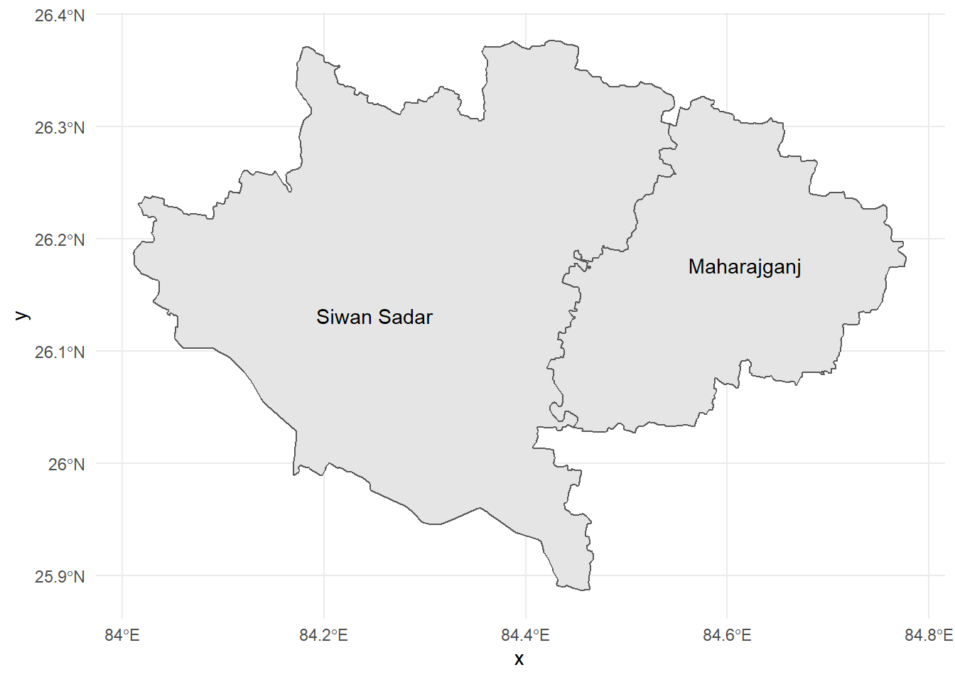

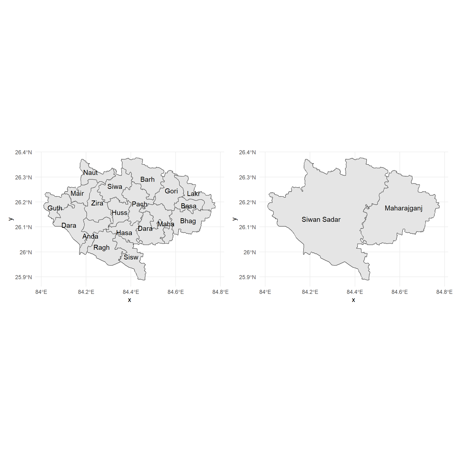
The transformation

(spatial_data %>% 
  ggplot()+
  geom_sf()+
  geom_sf_text(aes(label = str_sub(NAME,1,4)))+
  theme_minimal())+(spatial_data %>% 
  group_by(Anumandal) %>% 
  summarise(
    Number_of_Blocks = n()
  ) %>% 
  ggplot()+
  geom_sf()+
  geom_sf_text(aes(label = Anumandal))+
  theme_minimal())

## `summarise()` ungrouping output (override with `.groups` argument)

## Warning in st_point_on_surface.sfc(sf::st_zm(x)): st_point_on_surface may not
## give correct results for longitude/latitude data

## Warning in st_point_on_surface.sfc(sf::st_zm(x)): st_point_on_surface may not
## give correct results for longitude/latitude data